Bancreek Inflation Visualizer Methodology

The Bancreek CPI Item Analyzer is derived from five different raw data tables, all available at bls.gov:

·       cu.data.0.Current (“current”)

·       cu.data.1.AllItems (“all items”)

·       cu.series (“series”)

·       cu.item (“item”)

·       relative importance tables

The first four data tables are all published monthly at download.bls.gov - /pub/time.series/cu/. While we will not provide detailed descriptions of these databases in this post (for those looking for this, we’d refer you to another BLS text file you can access at the same link called cu.txt), we will briefly describe the general purpose of each file.

The current file is the main repository of all non-seasonally adjusted values for every item reported by the BLS. This is the engine of the dashboard, from which all year-over-year inflation/deflation calculations are derived.

The “all items” file is the same as current, except as the name suggests, it just houses the highest-level values for all items, rather than the values for each lower-level item on the hierarchy. We use this file to calculate the headline inflation number that is so widely reported each month.

The series and item files are used to “decode” the current and all items files as the latter two files only have codes (called “series id’s”) that are hard to interpret. The series file houses a field called the “item code”, while the item file houses the item name. Joining both files together with the current or all items files allows you know that, for example, the series id “CUUR0000SEFP01” is giving you the non-seasonally adjusted, regularly reported, all area code, nominal value for “coffee” in an given period.

Last is the relative importance tables. These tables provide the weighting factors for each item, and therefore are critical to the visualization which is relying on this data to size the impact of each unweighted change in item value. These tables are unfortunately not packaged as cleanly as the prior four data tables. To get all the relative importance data we needed to construct the visualization we had to collect the data one month at a time from the archived CPI releases .

In this section, we will step through the transformations we make to the raw data tables described in the prior section.

Item selection

The first decision we had to make is to choose the items to display within the tool. Our goal was to display the most granular set of items that totaled to 100%. Note that as of December 2023, there were 400 items in the items file. But we could not just display all 400 of these items as many of the items are collections of other items. In other words, with our goal being to build overall inflation up from its most granular components, we needed to find a set of items that summed to as close to 100% as possible. We undertook a manual process to choose the most granular set of items that would accomplish this goal. At the end of this process, we ended up with 179 distinct items. Note that it was not possible to achieve exactly 100% coverage through this process because the BLS has several “unmeasured” items in its hierarchy. While the unmeasured items are usually very small, as the name suggests they do not have measurements available monthly in the current file, but they do comprise a sliver of overall inflation. Without values in the current file, we could not capture the unmeasured items in our analysis. Having said that, over the 228 periods in our tool the 179 items that we are displaying are on average responsible for 99.10% of overall inflation. As such, we were pleased with the coverage we were able to achieve through this process.

Relative importance table creation

As mentioned in the prior section, we couldn’t locate a clean data table of historical relative importance values. As such, we had to create our own by pulling data down from each archived CPI news release. Beyond the time it took to manually download and format this data, the main challenge was that the archived CPI releases only provide relative importance by item names (rather than item codes). This was an issue because there have been multiple changes to item names over the period we wanted to present in this visualization. So, each time an item name changed, we had to remap the old item name to the new item name to ensure consistency over time. Most of the time the changes were obvious from inspection of the data – we could clearly see one series end and another start at almost identical weights. However, sometimes the mapping was less obvious. Nevertheless, we mapped all stale, unused historical item names to current item names to the best of our abilities. A summary of the mapping changes we used on the data is shown below:

Filling in gaps in current file

The last data cleaning step we took before we started joining data tables was to fill in gaps in the current file. In working with the current file, we started to notice that the total relative importance of all 179 items in some months were lower than other months. In researching this issue, we found some cases where the BLS did not report values in the current file for a handful of the 179 items we selected. We tried to see if the weight of the item that was not reported was grouped into a different item in those months but could not find any obvious outliers that would suggest this to be the case. As such, we decided to simply backfill any missing data at the 179 item code level with the most recently reported value. We figured at least this way we would have a rough estimate of inflation for the item code in the missing month, rather than just dropping it out of the data altogether.  

Data joining and manipulation

1. Join cleaned/backfilled current file to the series file to bring in item codes
2. Filter data to include only non-seasonally adjusted values for area code “0000”
3. Join relative importance values to the table from step 2
4. Calculate year-over-year changes in values for each item code
5. Offset the relative importance values properly to assign the correct relative importance value to survey month (note that the prior month’s relative importance values are reported in each BLS CPI release, so to assign the prior year’s relative importance values to any month, we had to offset relative importance by 11 months)
6. Calculate year-over-year inflation on the “all items” level to get headline inflation for all months. Join this together with data table from step 5
7. Join current item names to table from step 6
8. Calculate weighted change to inflation by multiplying unweighted change in value for each item by its prior year relative importance

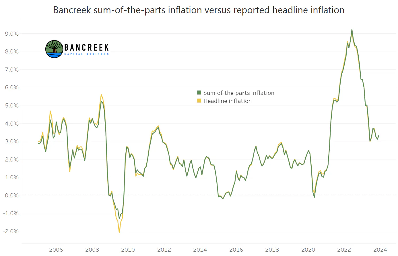
Again, the goal of this entire process was to be able to deconstruct inflation into its more granular components and use those components to quickly and cleanly display the drivers of inflation each month. Therefore, the main measure of success was to see if we were able to recreate headline inflation in each month by summing up our weighted inflation estimates at the item level. The following chart shows the comparison of our bottoms-up calculated inflation versus reported headline inflation:

Source: Bancreek Capital Advisors, LLC

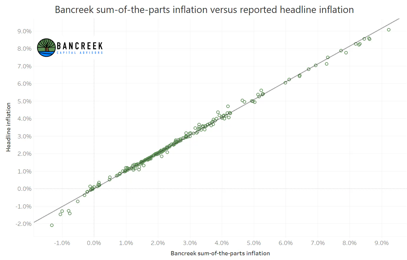
As shown above, the fit between our calculated inflation and reported headline inflation was quite close, especially after 2012, when the BLS changed its reporting practices to report changes in relative importance on monthly level (prior to March 2012 it was reported annually). We also found the R2 between our calculated inflation and the BLS’ reported inflation to be 0.99561, indicating an extremely close fit between the two data sets.

Source: Bancreek Capital Advisors, LLC

This validation exercise gave us confidence that the data transformations and assumptions described throughout this post were performed with enough accuracy to use as the basis for our visualizations.